|
<< Click to Display Table of Contents >> Algorithm |
  
|
|
<< Click to Display Table of Contents >> Algorithm |
  
|
Algorithm contains Logistic Regression, Decision Tree, K-Means Clustering, Association Rules and Time Series Analysis.
❖Logistic Regression
Logistic Regression is a type of disaggregated model for machine learning. Since the algorithm is simple and efficient, it is widely applied in practice.
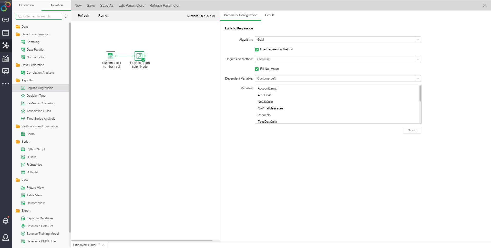
Drag a data set and a Logistic Regression node to the edit area. Connect the data set and Logistic Regression node. Selected Logistic Regression node setting and display area contain two pages: Parameter Configuration and Result.
oParameter Configuration
There are two algorithms for Logistic Regression: GLM and GLMNET. The default algorithm is GLM.
GLM:
Generalized linear model (GLM): This model takes linear prediction function of an independent variable as the estimated value of a dependent variable. It is often used in Logistic Regression.
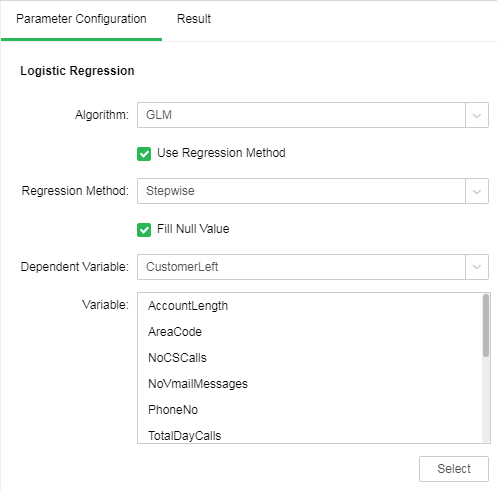
[Use Regression Method] Control whether the Regression method is used. It is default as selected.
[Regression Method] Include stepping, stepping forward and backward. It is default as stepping.
Stepwise: Build the equation step by step. The initial model is as simple as possible. The equation doesn't include any input field. In each step, evaluate the input fields which have not been added to the model. If the optimal input field can significantly enhance model prediction ability, the fields should be added to the model. In addition, the input fields contained in the model will be reevaluated to make sure that any field can be deleted when there is no significant loss to the model function. If yes, it can be deleted. And then, repeat this process. Add or remove other fields. The final model will be generated when no more fields can be added to improve the model, and no more fields can be deleted without reducing the model functionality.
Step Backward: Similar to the step-by-step method of stepping modeling. However, when this method is adopted, the initial model contains all the input fields as a predictive variable. The fields can only be deleted from the model. The input fields that have less impact on the model will be deleted one by one until no more fields can be deleted without significant damage to the model function thus to generate the final model.
Step Forward: Forward and backward are opposite Regression method. When this method is adopted, the initial model is the simplest model. It doesn't contain any input field. The fields can only be added to the model. The input fields not included in the model will be inspected in each step to see their effects on improving the model. After that, optimal fields will be added to the model. The final model will be generated when no more fields can be added or the best alternative fields can not significantly improve the model.
[Fill Null Value] Fill the mean value of the independent variables column to the column. The default is filling value.
[Dependent Variable] Select the fields used as dependent variable from the drop-down list. Any system (or model) is composed of various variables. When we analyze these systems (or models), we can choose to study the effects of some variables to others. Those variables we selected are known as independent variables, and those affected variables are referred to as dependent variables.
[Variable] Select the fields need to be used as independent variable from the selected column dialog box.
GLMNET:
GLMNET uses Lasso, Elastic-Net and other regularization modes to realize Logistic Regression.
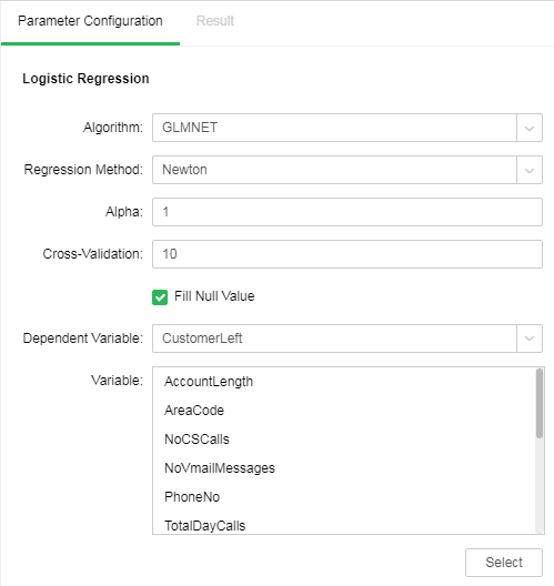
[Regression Method] Contains Newton method and quasi-newton method. Newton method is selected by default.
Newton method: A method of numerical optimization which utilizes the first-order and second-order derivatives of the function at the current point to search for direction.
Quasi-newton method: A deformation of Newton method which is a Hessian matrix using approximate matrix to substitute for Newton method.
[Alpha] Elastic-Net mix parameters. The value ranges from 0 to 1. When the value is equal to 1, penalty term adopts L1 norm; when the value is equal to 0, penalty term adopts L2 norm. The default value is 1.
[Cross-Validation] Optimal equation can be obtained through cross validation. The default value is 10.
oResult
1. Coefficient
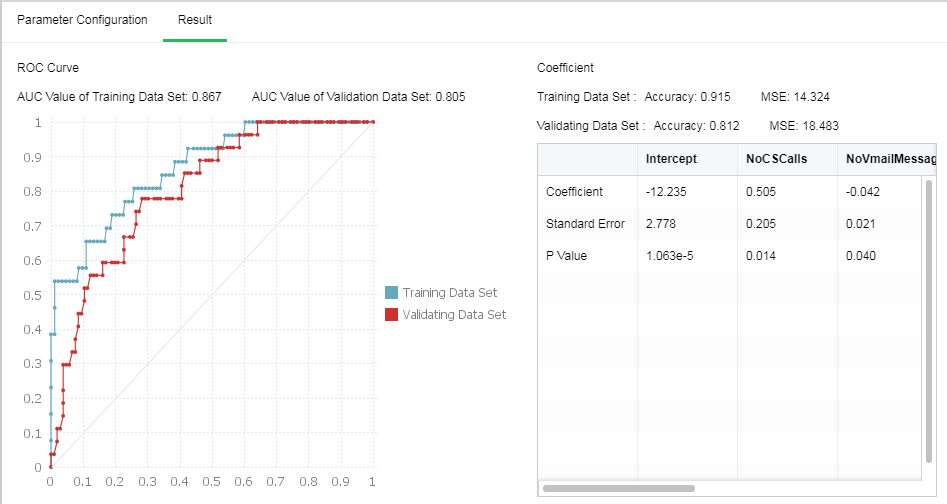
Using GLM algorithm, Logistic Regression equation coefficient can be obtained via model coefficient, including intercept term, coefficient of each independent variable, P value and standard error. Accuracy and mean square error after model training can be obtained. If data partition has been done, model accuracy and mean square error based on validation set can be seen. The following shows the results of GLM algorithm. If the coefficient is 0, the results will not be displayed in the model coefficient table.
2. ROC Curve
Prepare an ROC curve and calculate the AUC value. The higher the AUC value, the better the model classification effect will be. If data partition has been done, AUC values of validation sets can also be compared.
❖Decision Tree
Decision Tree is a tree structure used for example classification. Decision Tree is composed of nodes and directed edges. There are two node types: Internal node and leaf node. Among them, internal node represents testing conditions of a feature or attribute (Used to separate records with different characteristics). Leaf node represents a classification.
Once we have constructed a Decision Tree model, it is very easy to classify based on it. The specific method is as follows: Starting from the root node, test with a specific feature of the instance. Assign the instance to its child node according to the test structure (namely selecting an appropriate branch); if a leaf node or another internal node can be reached along the branch, perform recursive implementation by using new test conditions until a leaf node is reached. When reach the leaf node, we will get the final classification results.
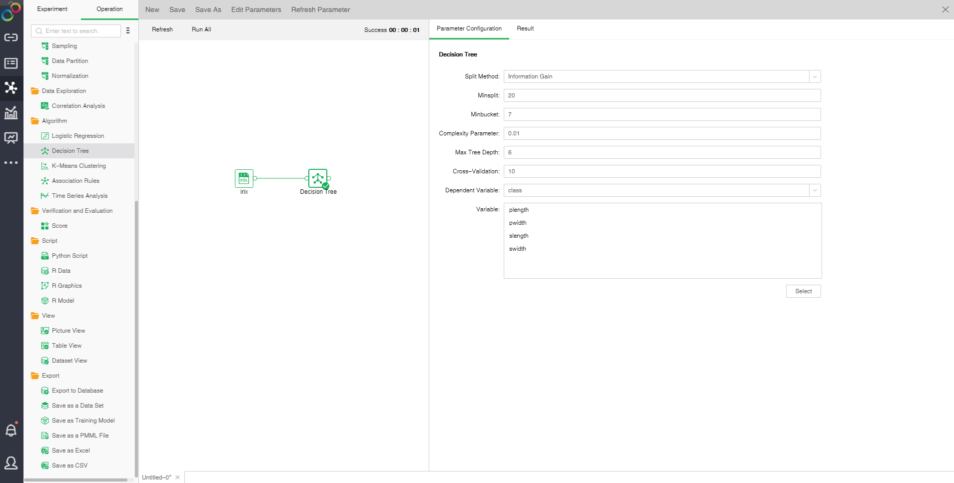
Drag a data set and a Decision Tree node to the edit area. Connect the data set and Decision Tree node. Selected Decision Tree node setting and display area contains two pages: Parameter Configuration and Result.
oParameter Configuration
[Split Method] Contains "Information Gain" and "Gini Coefficient."
Information gain: promoted value of the subset purity after division
Gini coefficient: probability of incorrectly assigning a sample randomly selected in a sample set
[Minsplit] If the sample number is smaller than the node, it will not be split. The default value is 20.
[Minbucket] If the sample number is smaller than the value, the branch will be cut off. The default value is 7.
[Complexity Parameter] Each division will calculate a complexity. When the complexity is greater than the parameter value, splitting will not be carried out any longer. The default value is 0.01.
[Max Tree Depth] Number of hierarchies of Decision Tree. The default value is 6.
[Cross-Validation] Optimal equation can be obtained through cross validation. The default value is 10.
[Dependent Variable] Select the fields used as dependent variable from the drop-down list. Any system (or model) is composed of various variables. When we analyze these systems (or models), we can choose to study the effects of some variables to others. Those variables we selected are known as independent variables, and those affected variables are referred to as dependent variables.
[Variable] Select the fields need to be used as independent variable from the selected column dialog box.
oResult
1. Tree Graph
There are two types of classification results, dichotomy and polytomy. When the dependent variable only has two different values, it is dichotomy; when the dependent variable has more than two different values, it is polytomy. Node ID is above the node. There are two rows within the node. The first row is the final classification of the node. In case of polytomy, the second row is the probability value of each classification of the node. In case of dichotomy, the second row is the probability value of the main classification of the node. Yes and no represent whether the conditions are met or not thus to determine the branch direction. Node color represents purity.
Binary tree form results are displayed as follows:
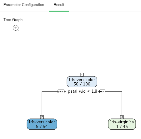
Note: A green node refers to the main classification. Blue node 5/54 indicates that Iris-versicolor is the probability value of Iris-virginica.
Polytomous tree form results are displayed as follows:
Click the zoom button to enlarge the image so that it can be viewed more clearly.
2. Summary of Node Classification
List the information of all leaf nodes.
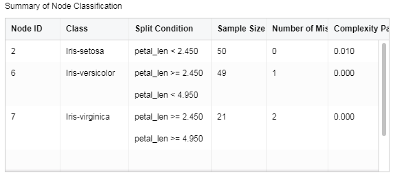
[Node ID] Number of lead node
[Class] Classification of lead node
[Split Comdition] Determination condition for root to leaf node
[Sample Size of Node] Sample number of leaf node
[Number of Misclassifications] Sample number of mis-classification
[Complexity Parameter] Complexity parameter of each leaf node.
3.Confusion Matrix
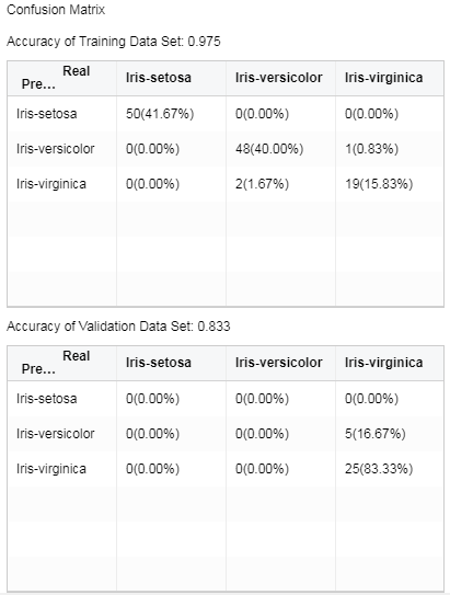
Situation analysis table of predicted results. In case of data partition, the analysis table of validation set can be checked.
The transverse header is the real value. And the vertical header is the predicted value. The integer value represents the number of samples, and the percent is the ratio of the number of samples to the total number of samples. The accuracy is the same proportion of the true value and the predicted value.
❖K-Means Clustering
K-Means is a type of Clustering algorithm, where K represents the number of classifications and Means indicates the mean value. Just as its name implies, K-Means is an algorithm for data Clustering via mean value. K-Means algorithm divides similar data points via the preset K value and initial Clustering center of each classification, and gets the optimal Clustering results via mean iterative optimization after division.
In order to enhance the computational efficiency of K-Means Clustering, Yonghong Z-Suite supports distributed system computing of K-Means. Distributed computing is used when the input node data set is "data mart data set."
Drag a data set and a K-Means Clustering node to the edit area. Connect the data set and K-Means Clustering node. Select "K-Means Clustering." The display area contains two tab pages, namely "Parameter Configuration" and "Result."
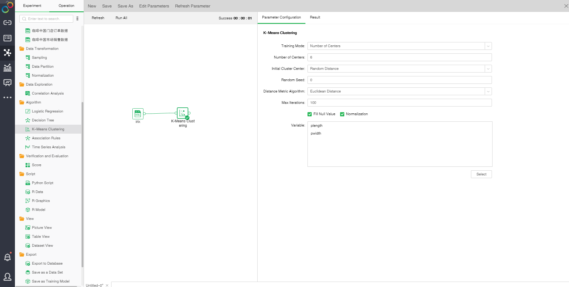
oParameter Configuration
[Training Mode] Contains number of Clustering center and range of the number of Clustering center
[Number of Centers] Number of Clustering center
[Centers Number Range] Range of the number of Clustering center.
[Initial Cluster Center] Initial Clustering center methods consist of random distance and Kmeans++. Random distance refers that all Clustering centers are randomly selected. In the Kmean++ method, the first Clustering center is randomly selected and other Clustering centers are selected according to distance. The farther away from the Clustering center, the higher probability will be.
[Random Seed] Generate random number seed. The default value is 0.
[Distance Metric Algorithm] Includes two methods: Euclidean distance and Cosine distance. Euclidean distance is the actual distance between two data points. Cosine distance is the measure between the cosine values of the two vetorial angles in vector space which is used to measure the difference between two individuals.
[Maximum Iterations] Maximum number of iterations. Calculate the stable number of Clustering center finally. The default value is 100.
[Fill Null Value] Fill the mean value of the independent variables column to the column. The default is filling value.
[Normalization] Normalizes independent variables. The default normalization method is Z-Score normalization.
[Variable] Select the fields need to be used as independent variable from the selected column dialog box.
oResult
The following figure shows the K-Means Clustering result in which the number of Clustering centers is 6 and the number of samples is 150.
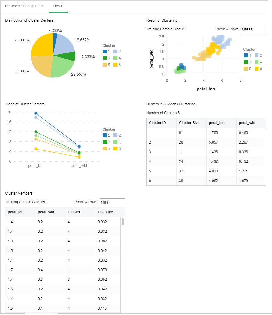
1. Distribution of Cluster Centers
The proportion of the number of samples in the cluster accounting in the total number of samples.
2. Trend of Cluster Centers
Variation tendency of each Clustering center on independent variable.
3. Result of Clustering
Scatter diagram after Clustering drawn based on the first two columns.
[Preview Rows] The chart displays 65535 rows of data by default. The value can be changed.
4. Centers in K-Means Clustering
Value of Clustering center on independent variable
5. Cluster Members
Sample cluster and distance to the Clustering center
[Preview Rows] The default number of preview rows is 1000. The value can be changed.
[Cluster] Classification number.
[Distance] Distance between each sample to the nearest Clustering center calculated according to distance calculating methods.
❖Association Rules
Association Rules is an unsupervised machine learning method. It detects the Association or correlation that may exist between objects behind data for knowledge discovery but not prediction. Such Association or relation is known as Rules.
Drag a data set and an Association Rules node to the edit area. Connect the data set and Association Rules node. Selected Association Rules node setting and display area contains two pages: Parameter Configuration and Result.
Association rules contain two algorithms: one is distributed FG-Growth, the other is non distributed Apriori.
•Apriori:

oParameter Configuration
[Range for Support (%)] Percentage range of the regular support level generated by the model. The Rules will be discarded if the value is not within the range.
[Confidence (%)] The minimum percentage value of the regular confidence level generated by the model. If the regular confidence level generated by the model is lower than the quantity, the Rules will be discarded.
[Minimum Length] Minimum item number generated by the model. It will be discarded if it is smaller than the value.
[Maximum Length] Maximum item number generated by the model. It will be discarded if it is greater than the value.
[Variable] Select the fields need to be used as independent variable from the selected column dialog box.
oResult
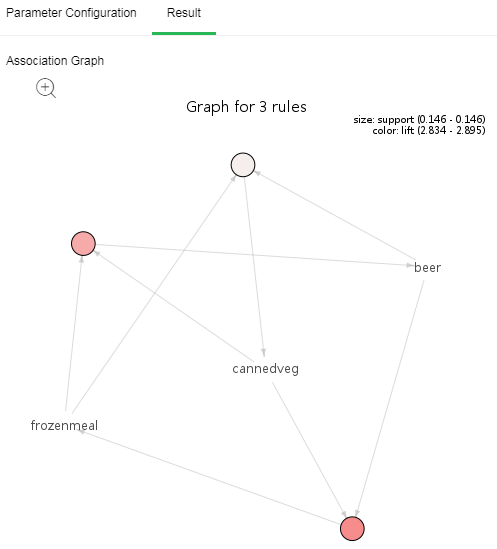
1. Association Graph
Association Graph of each item. Each circle represents a rule. The ones pointing to the circle are left items, and the ones pointed by the circle are right items; the circle size represents the supporting degree. The bigger circle, the higher supporting degree will be. Circle color represents promotion degree. The deeper the color, the higher promotion degree will be.
Click the zoom button to enlarge the image so that it can be viewed more clearly.
2. Association Rules
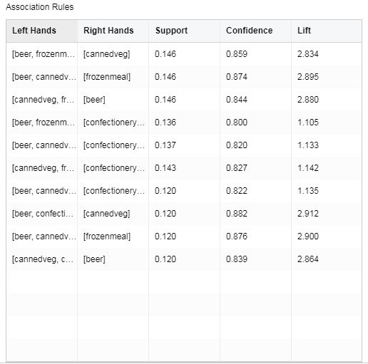
[Left Hands] Regular forerunner item set
[Right Hands] Regular conclusion item set
[Support] The number of occurrence of the item set divided by the total number of records
[Confidence] The number of occurrence of the item set {X,Y} divided by the number of occurrence of the item set {X}.
[Lift] Independence of measure item set {X} and item set {Y}. The higher the value, the better the model will be.
•FG-Growth
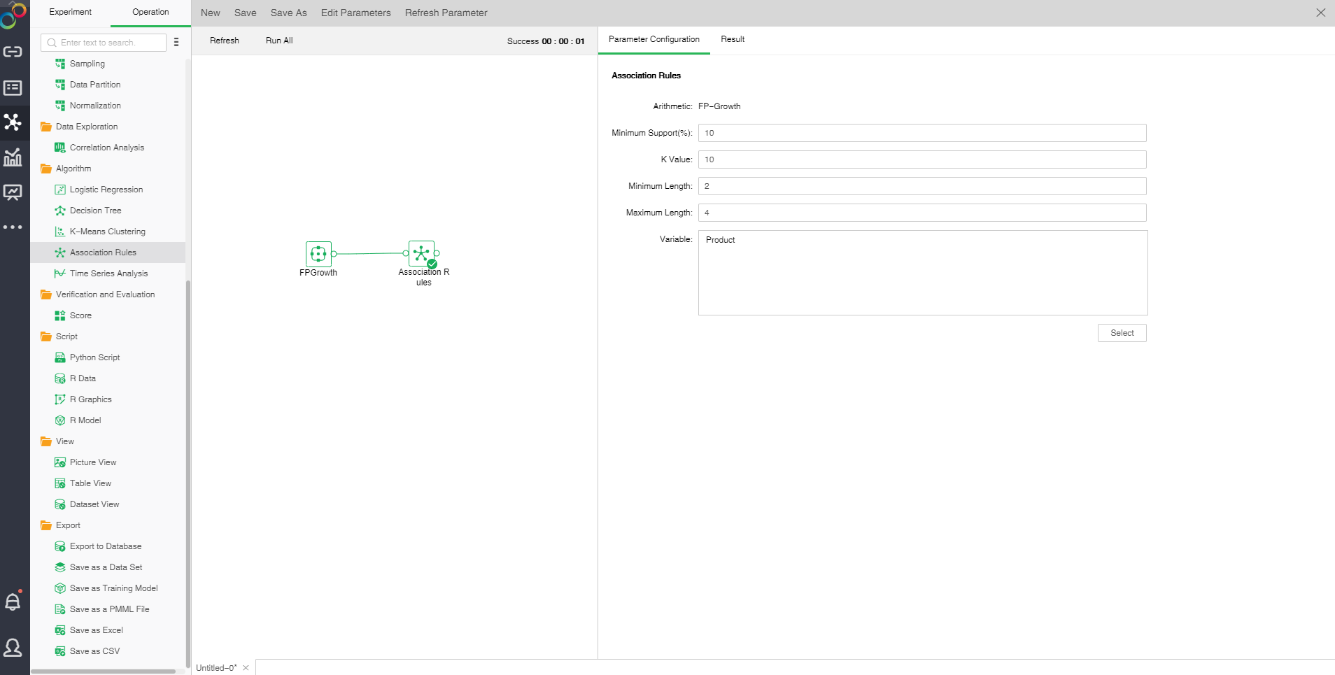
oThe configuration of Association Rules model
After adding the association rule model to the experiment, the model can be set up through the "configuration project" page on the right.
[Minimun Support(%)]Minimum support is used to measure the frequency of a set in the original data. If the rules are not in this range, the rules will be abandoned.
[K Value]the number of rows displayed by the model generated by the model.
[Minimum Length]number controls minimum length of frequent itemsets, less than this value will be discarded.
【Maximum Length】controls the maximum length of frequent itemsets, greater than this value will be discarded.。
【Variable】select fields from the selection column dialog box as independent variables.
oResult
After the successful operation of the Association Rule model, the result of the experimental model can be viewed through the "result display" page on the right side.
1. Association Rules
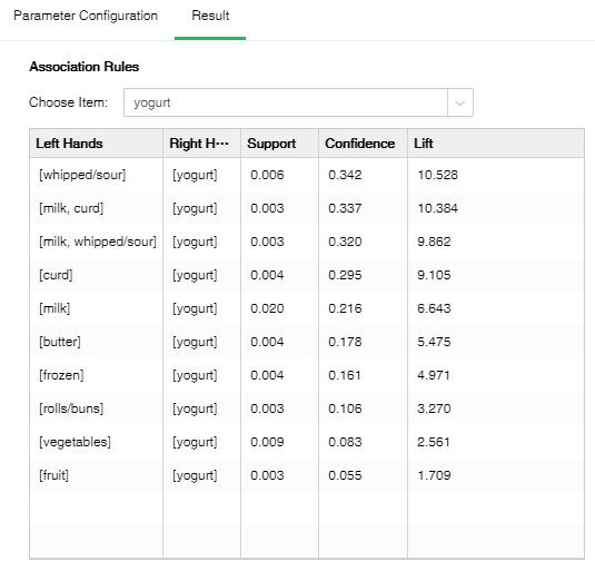
[Choose item] one of the item names contained in the fields in the database.
[Left Hands] The set of leading items of the rule.
[Right Hands] The set of conclusion items of the rule.
[Support] The number of occurrences of the item set divided by the total number of records.
[Confidence] The number of occurrences of the item set {X,Y} at the same time accounts for the proportion of occurrences of the item set {X}.
[Lift] Independence of measure item set {X} and item set {Y}. The larger the value, the better the model.
❖Time Series Analysis
Time Series Analysis carries out analysis of the sampling data for a period of time at constant duration by taking horizontal and seasonal trends into consideration to forecast data for a period of time in the future. That is, predict the future data based on the known historical data.
Drag a data set and a Time Series Analysis node to the edit area. Connect the data set and timing analysis node. Selected Time Series Analysis node setting and display area contain two pages: Parameter Configuration and Result.
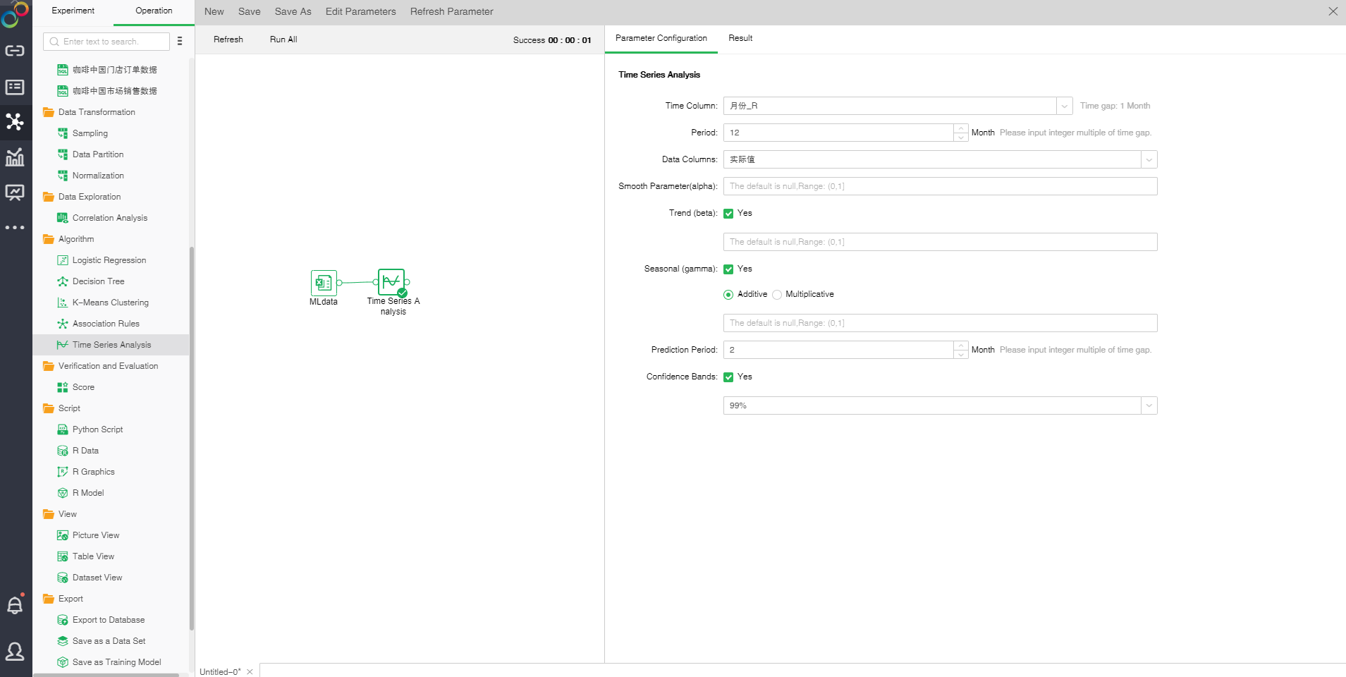
oParameter Configuration
[Time Column] Select time field. Automatically calculate the time interval according to the selected time field data.
[Period] Integer multiples of the time interval are required. Calculate the frequency depending on the period and time interval (period/time interval), namely the number of observations per unit time. The system will automatically fill in a reasonable value to a circle according to the time interval. The value can be manually modified.
[Data Columns] Selected data field
[Smooth Parameter (alpha)] The closer α is to 1, the closer to current data value the value after smoothing will be.
[Trend (beta)] Indicates whether longitudinal trend is considered or not. It is clicked by default which indicates fitting according to longitudinal trend.
[Seasonal (gamma)] Indicates whether seasonal trend is considered or not. If it is not selected, non-seasonal model fitting is enabled. If it is set as clicking, carry out seasonal model fitting. A seasonal pattern can be additive or multiplicative. Additive is clicked by default which indicates growth according to the trend of seasonal additive. If "Multiplicative" is checked, it indicates a growth in the trend of seasonal multiplicative. In case of seasonal model fitting, there should be at least two data points within a period. That is, the frequency is equal to or greater than 2, and the time series contains at least two periods.
[Prediction Period] Indicates the time span for backward prediction. The value should be in integral multiple of time interval. After select the time column, the system will automatically fill in a reasonable value which can be manually modified.
[Confidence Bands] Calculate the upper and lower limits of the estimated value based on the level. The default level is 99%.
oResult
1. Seasonal Model Prediction Curve
[History Fitted] Historical data changing curve and fitting data changing curve. The green line indicates historical data changing curve; the black line indicates fitting data changing curve. The higher overlap ratio of the two lines, the higher fitting ratio will be.
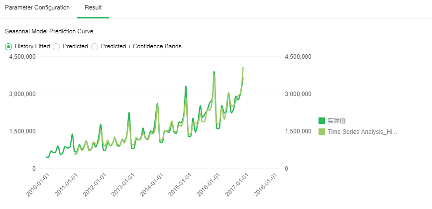
[Predicted] Prediction within specified deadline in the future. The green line indicates historical data changing curve; the black line indicates prediction changing curve within specified deadline in the future. This shows the variation trend of data in the future.
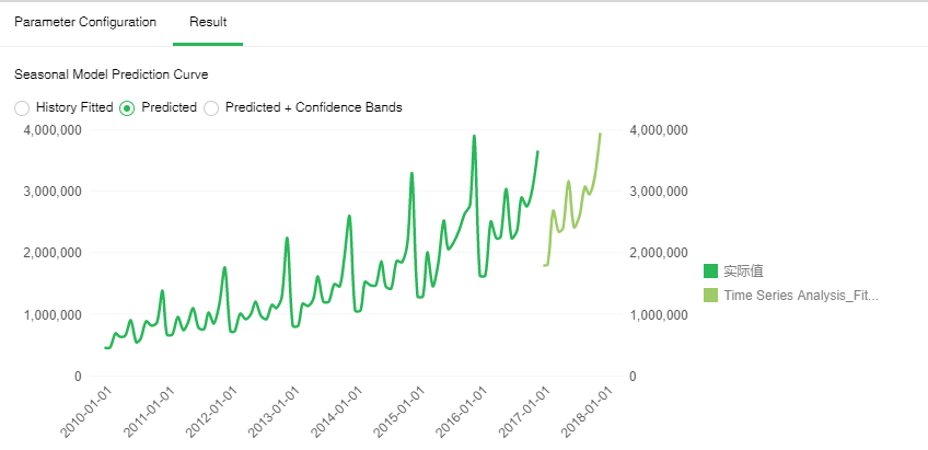
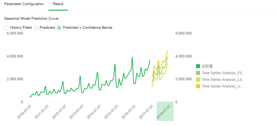
[Predicted + Confidence Bands] Prediction within specified time segment in the future. The dark green line indicates historical data changing curve; the black line indicates prediction changing curve within specified deadline in the future. The light green line is the upper limit of the confidence interval, and the orange line is the lower limit of the confidence interval.
2. Model Statistics
[MAPE] MAPE (mean absolute percentage error) reflects the relative value of error and is used for estimating a model. Generally, a model with the MAPE value less than 20 is a good model.
[Ljung Box Q-test] A type of statistical test to check whether time series has any lag correlation. If the significance is less than 0.05, the error has obvious self-correlation which indicates poor model fitting. The closer the significance value is to 1, the better model fitting will be.
