<< Click to Display Table of Contents >> Current:  Advanced Analytics > Experiment and Application of Advanced Analytic > Y-Advanced Analytics  Time Series Analysis

❖Financial forecasting

Time series analysis is to carry out analogy according to the development process, direction and trend reflected by time series and to predict the development law of the next stage. The enterprise can timely and effectively monitor the financial risk of the enterprise through time series analysis model.

 

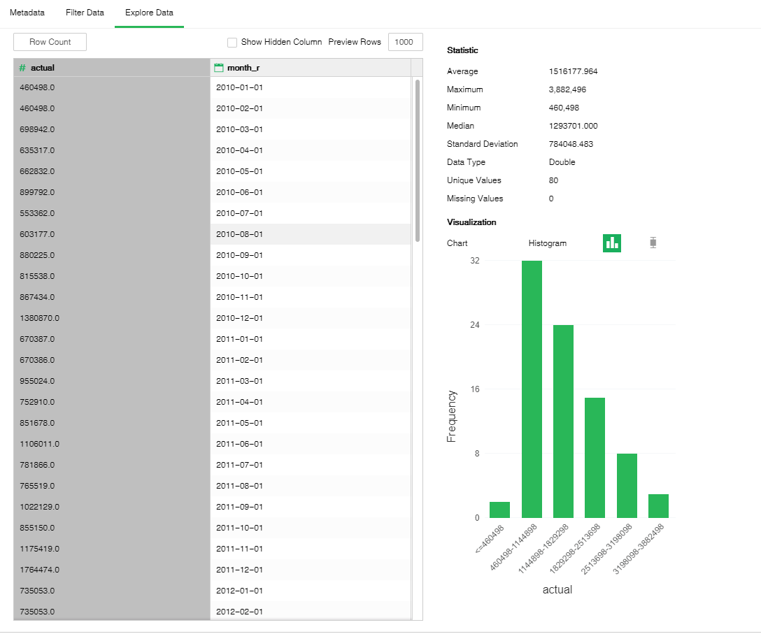
•Data Exploration

Drag the data set node "Financial Data" to the edit area. Select the actual value on the "Explore Data" page. Analyze monthly financial income distribution from 2010 to 2016 via histogram.

 

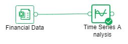
•Time Series Analysis

Drag Time Series Analysis node and connect to data set node.

 

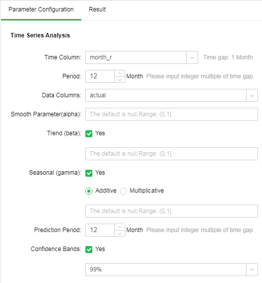
oConfiguration items

Select Time Series Analysis node configuration parameters as shown below:

oRunning

Click Run All.

 

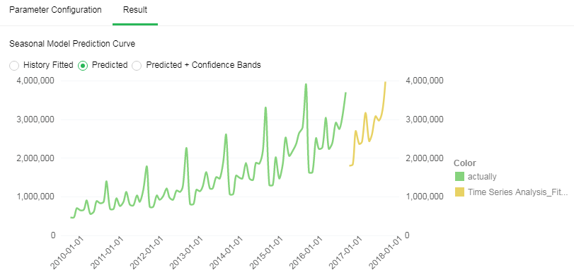
•Results analysis

oFitting degree analysis

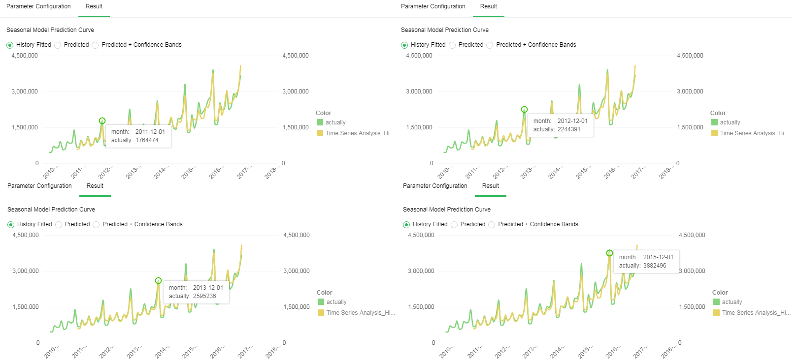
The green part in the diagram is the actual value and the gray line indicates fitting value. The figure below shows that the overlap ratio of fitting curve and actual curve is quite high which indicates that model prediction is quite successful. The peak value prediction is quite accurate.

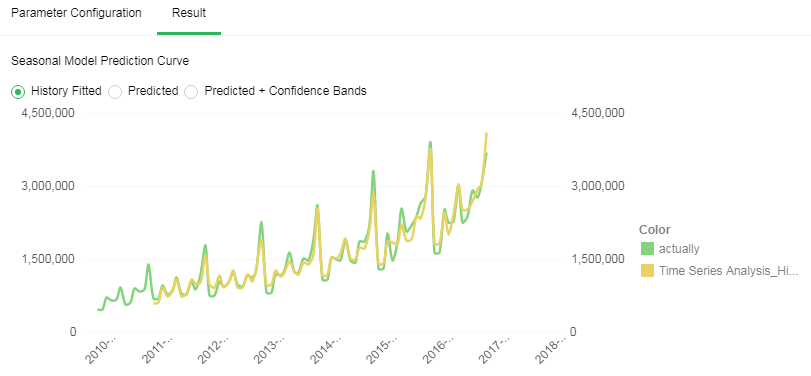
oDistribution instruction 

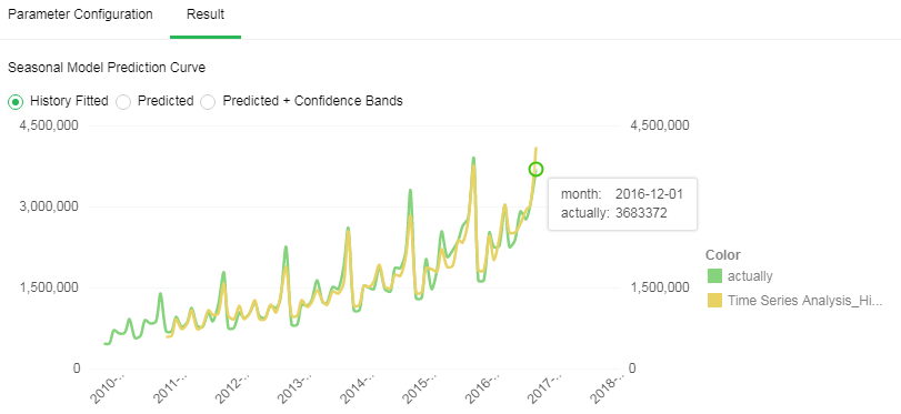
The figure shows yearly increasing of the overall trend. Higher index trend appears at the end of each quarter. It is especially obvious at the end of a year. 

 

But in December 2016, it is subject to significant fluctuation. The actual income is obviously lower than the level of the same period. It may be affected by the policy or macroeconomic environment.

oModel statistics description

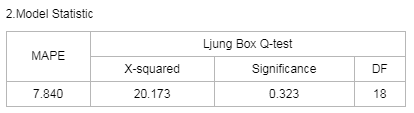
[MAPE] MAPE (mean absolute percentage error) reflects the relative value of error and is used for estimating a model. Generally, a model with the MAPE value less than 20 is a good model.

[Ljung Box Q-test] A type of statistical test to check whether time series has any lag correlation. If the significance is less than 0.05, the error has obvious self-correlation which indicates poor model fitting. The closer the significance value is to 1, the better model fitting will be.

oPredicted value analysis

 

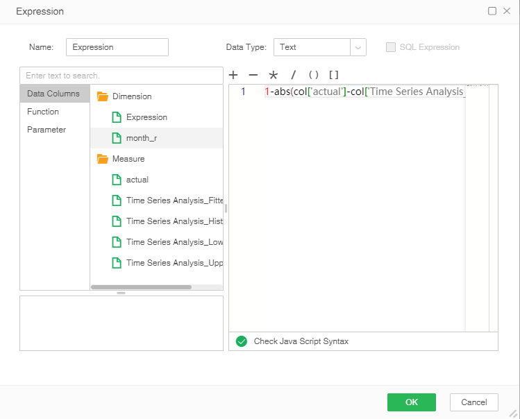
▪Analysis of data fitting accuracy

1. Connect the "Time Series Analysis" node and save  as a Data Set.

2.On the "Create Data Set" page, open the saved embedded data set. In the "Metadata" area, right-click "Create Expression" and choose "Accuracy" from the context menu. Input script: 1-abs(col['actual value']-col['Time Series Analysis _ historical fitting value'])/col['timing analysis _ historical fitting value']

3.Compare the actual value and historical fitting value of the financial figures of 2015 and 2016. It is detected that the prediction accuracy is quite high. The average accuracy is 91.34%. The prediction average accuracy of 2016 is 93%.

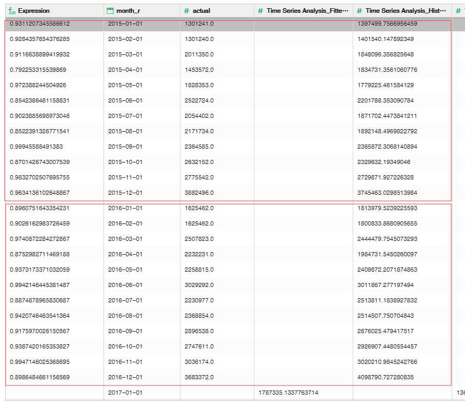
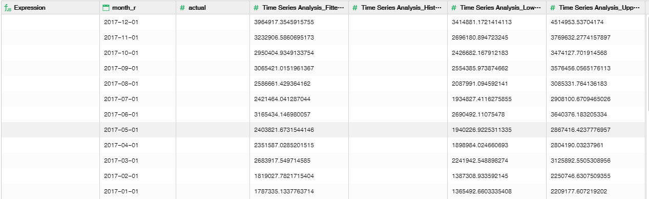
▪Model prediction value

The following figure shows the prediction value of 2017.