|
<< Click to Display Table of Contents >> Logistic Regression |
  
|
|
<< Click to Display Table of Contents >> Logistic Regression |
  
|
Logistic Regression is a type of disaggregated model for machine learning. Since the algorithm is simple and efficient, it is widely applied in practice.
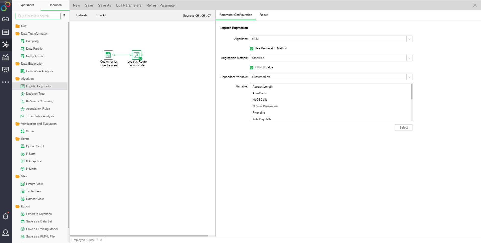
Drag a data set and a Logistic Regression node to the edit area. Connect the data set and Logistic Regression node.

❖Configuration of Logistic Regression model
After adding the Logistic Regression model to the experiment, you can set the model through the "Parameter Configuration" page on the right side.
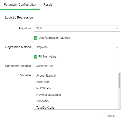
There are two algorithms for Logistic Regression: GLM and GLMNET. The default algorithm is GLM.
•GLM
Generalize dlinear model(GLM): This model takes linear prediction function of an independent variable as the estimated value of a dependent variable. It is often used in Logistic Regression.

[Use Regression Method] Control whether the regression method is used. It is default as selected.
[Regression Method] Include stepping, stepping forward and backward. It is default as stepping.
•Stepwise: Build the equation step by step. The initial model is as simple as possible. The equation doesn't include any input field. In each step, evaluate the input fields which have not been added to the model. If the optimal input field can significantly enhance model prediction ability, the fields should be added to the model. In addition, the input fields contained in the model will be reevaluated to make sure that any field can be deleted when there is no significant loss to the model function. If yes, it can be deleted. And then, repeat this process. Add or remove other fields. The final model will be generated when no more fields can be added to improve the model, and no more fields can be deleted without reducing the model functionality.
•Step Backward: Similar to the step-by-step method of stepping modeling. However, when this method is adopted, the initial model contains all the input fields as a predictive variable. The fields can only be deleted from the model. The input fields that have less impact on the model will be deleted one by one until no more fields can be deleted without significant damage to the model function thus to generate the final model.
•Step Forward: Forward and backward are opposite regression method. When this method is adopted, the initial model is the simplest model. It doesn't contain any input field. The fields can only be added to the model. The input fields not included in the model will be inspected in each step to see their effects on improving the model. After that, optimal fields will be added to the model. The final model will be generated when no more fields can be added or the best alternative fields can not significantly improve the model.
[Fill Null Value] Fill the mean value of the independent variables column to the column. The default is filling value.
[Dependent Variable] Select the fields used as dependent variable from the drop-down list. Any system (or model) is composed of various variables. When we analyze these systems (or models), we can choose to study the effects of some variables to others. Those variables we selected are known as independent variables, and those affected variables are referred to as dependent variables.
[Variable] Select the fields need to be used as independent variable from the selected column dialog box.
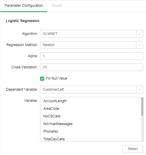
•GLMNET
GLMNET uses Lasso, Elastic-Net and other regularization modes to realize Logistic Regression.

[Regression Method] Contains Newton method and quasi-newton method. Newton method is selected by default.
Newton: A method of numerical optimization which utilizes the first-order and second-order derivatives of the function at the current point to search for direction.
Modified-newton: A deformation of Newton method which is a Hessian matrix using approximate matrix to substitute for Newton method.
[Alpha] Elastic-Net mix parameters. The value ranges from 0 to 1. When the value is equal to 1, penalty term adopts L1 norm; when the value is equal to 0, penalty term adopts L2 norm. The default value is 1.
[Cross-Validation] Optimal equation can be obtained through cross validation. The default value is 10.
❖Running experimental model
When the user completes the configuration of the model, clicking on the logical regression node and selecting "run" in the right menu, the model can run, and the running time is calculated at the top right of the edit area. You can also directly click the "run all" above the edit area to run the experimental model you set.
After the operation is successful, the output of the box will be output. Click the contraction icon to check the node state and display the node successfully, as shown in the following figure.

If the operation fails, the node will prompt failure. If the mouse is hung on the node, it can see the cause of failure, as shown in the following figure.

❖Result
After the successful operation of the Logistic Regression model, we can see the result of the experimental model through the "Result" page on the right side.
•Coefficient
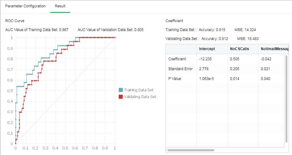
Using GLM algorithm, Logistic Regression equation coefficient can be obtained via model coefficient, including intercept term, coefficient of each independent variable, P value and standard error. Accuracy and mean square error after model training can be obtained. If data partition has been done, model accuracy and mean square error based on validation set can be seen. The following shows the results of GLM algorithm. If the coefficient is 0, the results will not be displayed in the model coefficient table.
•ROC Curve
Prepare an ROC curve and calculate the AUC value. The higher the AUC value, the better the model classification effect will be. If data partition has been done, AUC values of validation sets can also be compared.

❖Save as a trained model
After the successful operation of Logistic Regression model, we can choose to connect "Save as Trained Model" node and run . Only if the Logistic Regression model is saved as training model, can we make visual application in making report module. In the directory of the left training model, we can see the Logistic Regression training model.
Taking "Examples/Customer Losing" as an example, we select the logical regression node, and the node configuration project is as follows:
Save as a training model, and open the saved training model. The information is displayed as follows:
|
❖Export PMML
When the model node has been trained , the corresponding PMML file will be generated. Users can choose to connect "Save as a PMML File" node then run it, and export the generated PMML file to the local area, and then use it for other platforms.
❖Logical regression node rename
In the right-click menu of the logical regression node, select "Rename" to rename the node.
❖Deleting the logical regression node
In the right button menu of the logical regression node, select "Delete" or click the keyboard delete key to delete. It can delete the node and the input and output connection of the node.
❖Refresh the logical regression node
In the right-click menu of the logical regression node, select "Refresh" to update synchronous data or parameter information.