<< Click to Display Table of Contents >> Current:  Advanced Analytics > Old Operation > Algorithm  Time Series Analysis

Time Series Analysis is to carry out analogy according to the development process, direction and trend reflected by time series and to predict the development law of the next stage. The enterprise can timely and effectively monitor the financial risk of the enterprise through Time Series Analysis model.

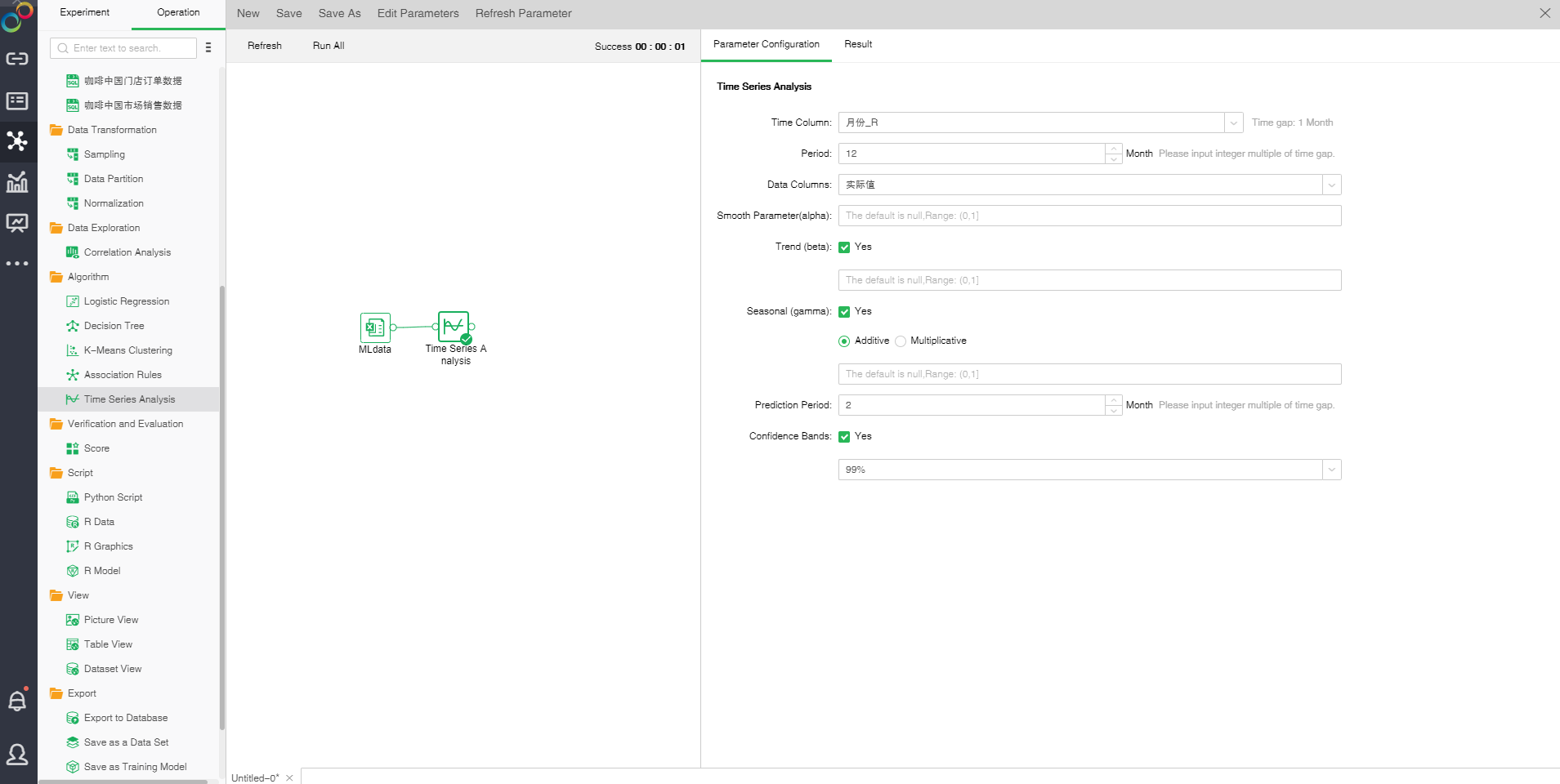
Drag a data set and a timing analysis node to the edit area to connect the data set and the timing analysis node. Selected timing analysis node settings and display area contains two pages: configuration items, results display.

 

 

❖The configuration of Time Series Analysis model

[Time Column] Select the time field. Based on the data of the selected time field, the time interval is automatically calculated.

[Period] needs to be filled in multiples of the time interval, and the frequency is calculated according to the period and time interval (period/time interval), ie the number of observations per unit time. According to the time interval, the system will automatically enter a reasonable value into the cycle, this value can also be manually modified.

[Data Columns] Select the data field.

[Smooth Parameter (alpha)] The closer ??is to 1, the closer the smoothed value is to the current time data value.

[Trend(beta)] Whether to consider vertical trends. The default is checked, indicating a vertical trend fit.

[Seasonal(gamma)]Whether gamma considers seasonal trends. If set to FALSE, no seasonal model fits. If set to check, seasonal model fitting is performed. Seasonal patterns can be additive and multiplicative. The additive effect is checked by default, indicating that the trend of seasonal addition increases. When the multiplication effect is checked, it indicates an increase in seasonal multiplication trends. When fitting a seasonal model, it is necessary to satisfy at least two data points in one period, that is, the frequency is greater than or equal to 2 and the time series contains at least 2 periods.

[Prediction Period] The time span for future forecasting needs to be filled with an integral multiple of the time interval. After selecting the time column, the system will automatically fill in a reasonable value, this value can also be manually modified.

[Confidence Bands] Calculates the upper and lower bounds of the estimate based on Level. The default Level is 99%.

 

❖Run the experimental model

When the user completes the configuration of the model, click the Timing Series Analysis node, and the right key menu selects "run" to run the model. After starting the operation, the editing area starts to calculate the running time in the upper right. You can also directly click the "run all" above the edit area to run the experimental model you set.

After the operation is successful, the output of the box will be output. Click the contraction icon to check the node state and display the node successfully, as shown in the following figure.

If the operation fails, the node will prompt failure, hover over the node to see the reason for the failure, as shown below.

 

❖Result

•Seasonal Model Prediction Curve

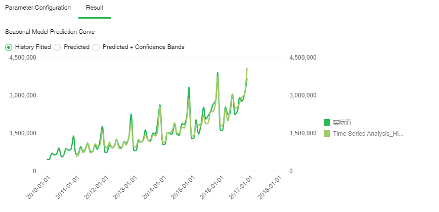
[History Fitted] Historical data change curve and fitting data change curve. The green line is the historical data change curve, and the light green line is the fitting data change curve. The higher the coincidence of the two lines, the better the fit.

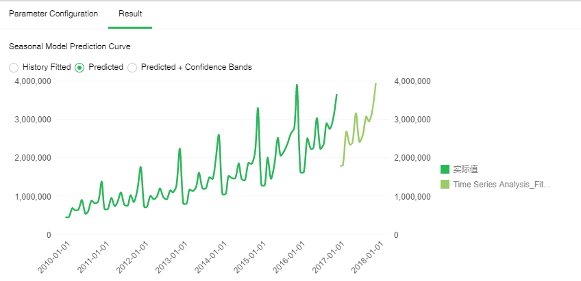
[Predicted] Forecasts for the specified period of time in the future. The green line is the historical data change curve, and the light green line is the predicted change curve for the specified time period. From this we can see the trend of future data changes.

 

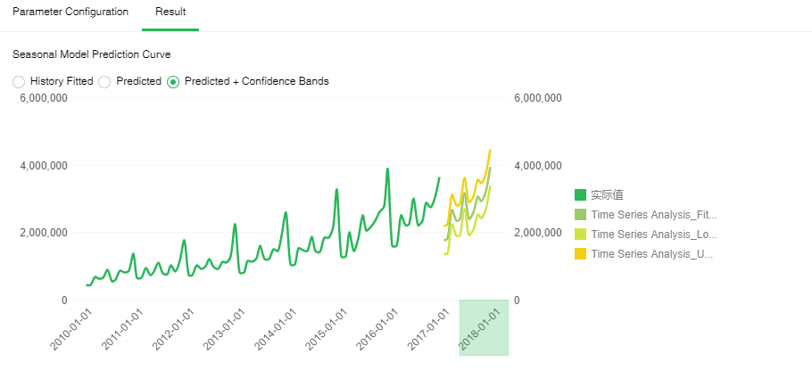
[Predicted+ Confidence Bands] Forecasts for future specified time periods. The dark green line is the historical data change curve, and the light green line is the predicted change curve in the specified time period. The yellow line is the upper bound of the confidence interval, and the orange line is the lower bound of the confidence interval.

 

•Model Statistic

[MAPE] MAPE (mean absolute percentage error) reflects the relative value of error and is used for estimating a model. Generally, a model with the MAPE value less than 20 is a good model.

[Ljung Box Q-test] A type of statistical test to check whether time series has any lag correlation. If the significance is less than 0.05, the error has obvious self-correlation which indicates poor model fitting. The closer the significance value is to 1, the better model fitting will be.

 

❖Save as trained model

After the timing analysis model runs successfully, we can choose to connect "Save as Trained Model" node and run . Only when the model is saved as a training model, the application of the report module can be visualized.

 

❖Save as a data set

Data less than 100,000 can be saved as embedded data sets, and over 100,000 are not allowed to be saved as embedded data sets. Saved data sets can be viewed in the Create Data Sets module.

 

❖Export to database

Imports the node data into the table specified by the selected database.

 

❖Renaming a timing analysis node

In the right-click menu of the timing analysis node, select "Rename" to rename the node.

 

❖Delete timing analysis node

In the right-click menu of the timing analysis node, select "delete" or click the delete key on the keyboard to delete the input and output connections of nodes and nodes.

 

❖Refresh timing analysis node

In the right-click menu of the timing analysis node, select "Refresh" to update the synchronization data or parameter information.