<< Click to Display Table of Contents >> Current:  Create Dashboard > Table > Visual Analysis  Highlight

Highlight can be set in the output component. Highlight is to make the matching data be displayed in the set color, font, background or format, so as to distinguish it from other data on the display. Select  the data area of the table, the mark of the chart, the text of the bound data, the data area of the pivot,  the cells of the freestyle table, and the gauge, and the highlight option in the general of the right panel . If the user has bound date and profit data segments on the chart component, the mark is displayed in red when the profit is negative. When you copy a component, highlighting is also copied.

 

❖Highlight Areas Of Different Components

Highlight is defined for specific areas of a component.

 

❖How to Use

1. Select the area where you want to highlight, and click the highlight option in the set up of the right panel to open the highlighted dialog. The highlight dialog of the chart can only set the background color. The highlight dialog of the table, pivot, freestyle table, text and gauge components can set the font and background color, as well as set the data format, as shown in the following figure. By default, the format is empty. Options include: date, number, currency, percent, text and so on. Among them, the text supports user-defined display types. The format setting method in the highlighting is similar to the format set in the local format. For details, see the format description.

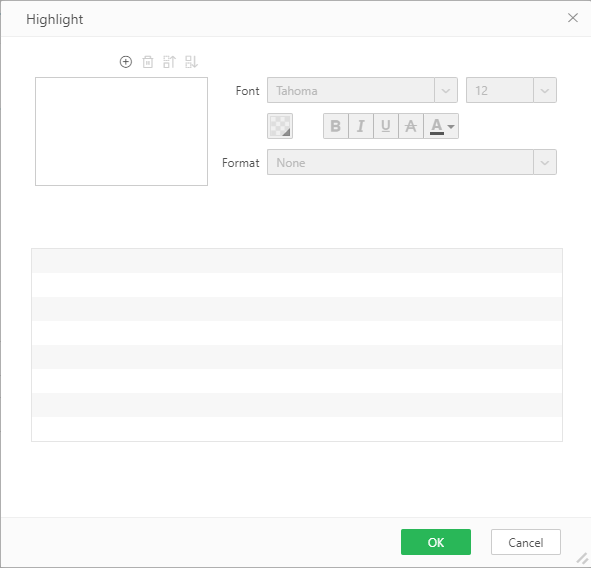
Select the table component cell and click the highlight in the general of the right panel to open the highlight dialog. If no new highlight is selected, the options will be disabled, as shown in the following figure.

 

2.Clicking the Add button on the opened highlight dialog will add a highlight condition. The default name is "highlight". The user can modify the name. After setting, click the blank to take effect. The user can add multiple highlights and set the display order of different highlight conditions by moving the buttons up and down.

3.The background color, foreground color, font style, and text format can be set for the highlight condition. Note that there are no foreground and font settings in the highlighted dialog on the chart, because there is no meaning for the mark. Formatting methods are similar to those in the component's local format.

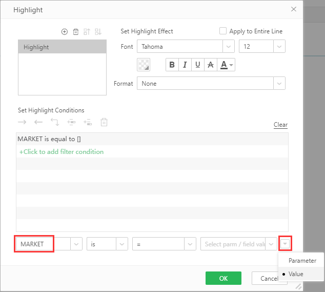
4.Click the row of "click to add filter condition" or right-click "add filter condition" in the table to create a new highlighted filter condition. The detailed introduction of setting filter condition is in the filter section. However, when setting filter conditions, only bound data segments can be set with conditions, and only dimension data segments can display corresponding values, as shown in the figure below. After selecting the mark column, select the field value, and the value corresponding to mark will be displayed in the value drop-down list.

5. Click the OK button, highlighting will take effect.

 

❖Special Uses of Highlight in Table, Pivot and Freestyle Table

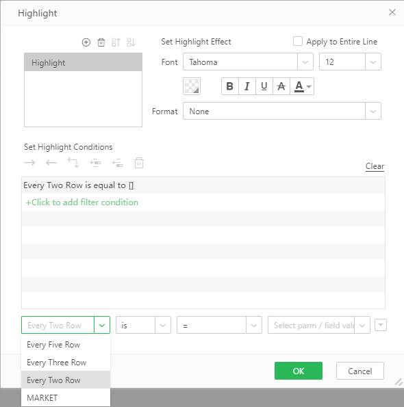
You can set the style of the component every two row, every third row, and every five row  by parameters on the table component, pivot, and freestyle table components.

 

Parameter setting:

Parameters optional at every two rows only include 0 and 1.

Parameters optional at every three rows include 0, 1 and 2.

Parameters optional at every five rows include 0-4.

 

➢For Example: Explaining at  every two rows.

When setting the filter condition on the "Sum_AREA_CODE" data area of the table component to every two row, it is equal to 0, and the background color is set to yellow, set the format to numeric type "#,###K".

 

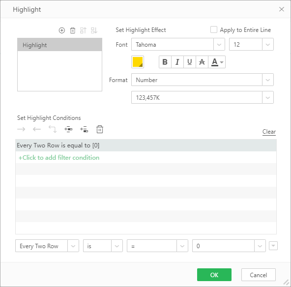
Then, all the even-numbered rows in the data area satisfy the filter condition. Note that the header of this column also participates in the parity operation.

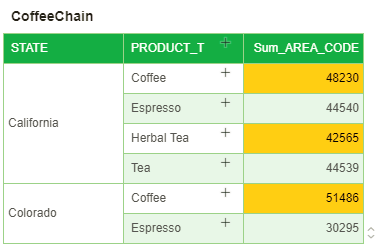
The result of the execution is shown in the figure below:

 

❖Special Uses of Highlights in Table

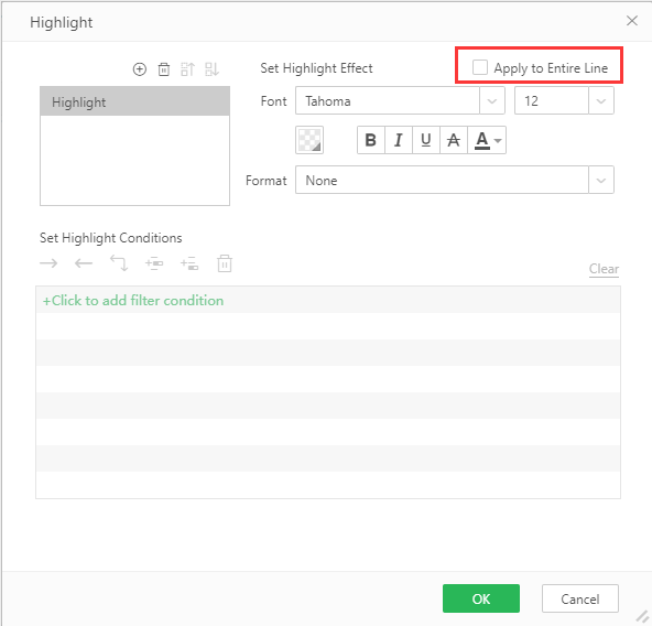
Highlight applied to the whole line function: after adding a highlight to the table component, click the blank area, and the [apply to whole row] function will be displayed in the upper right corner, as shown in the figure below; you can select whether to check, if you check, the current highlighted effect will be applied to the whole row.

Be careful:

1. If the highlight applied to the whole row is checked, it is called the row highlight; if it is not checked, it is called cell highlight.

2. Row highlighting always ranks below the cell highlight in the highlighted dialog, that is, the rendering priority of row highlighting is always lower than that of cell highlighting.

 

❖Example:How to Use Highlight

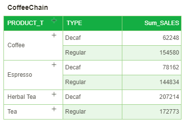
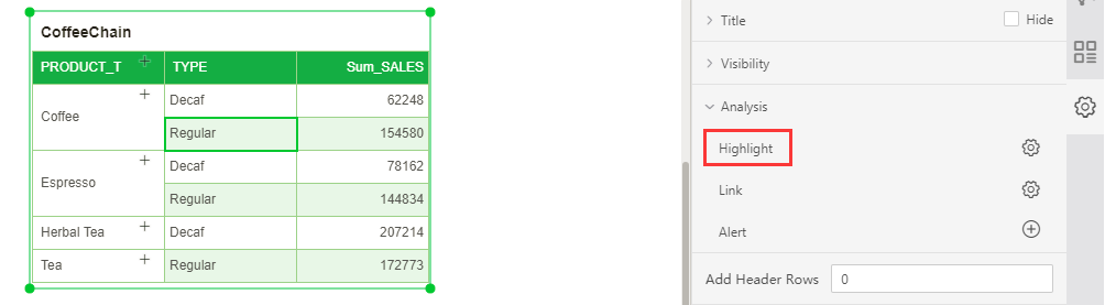
1. Create a new table and bind the data shown in the figure below.

2. Select the second column data area and click the highlight in the general of the right panel , as shown below:

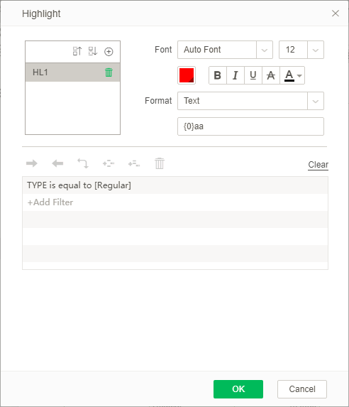
3. Add highlighted in the highlight dialog , set the highlighted name as HL1, then set the highlighting condition TYPE is equal to Regular, set the background color to red, formatted as text format "{0}aa", as follows Picture shows.

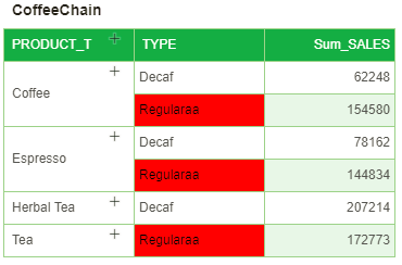
4. Click the OK button, the cell with TYPE of Regular in the table is highlighted, the cell background is red and the text is displayed as Regularaa. As shown below.

 

❖Set the Format of Null Value by Highlight Function

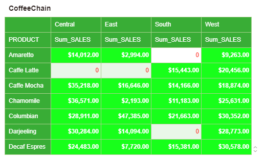
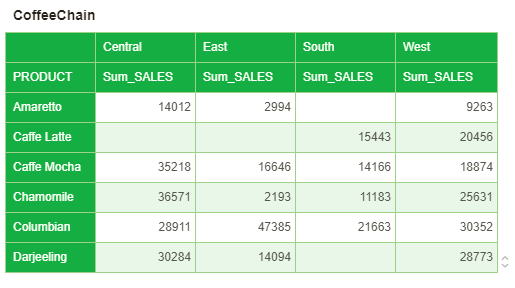
1. Create a new pivot. The binding data is as shown in the following figure:

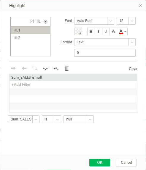
2. Select the summary cell area, open the highlight dialog in the right panel, add two highlights, the name is "HL1" and "HL2", set HL1: font color is red, set the format to text format, The value is "0" and the filter condition is "Sum_SALES" is "null", as shown below.

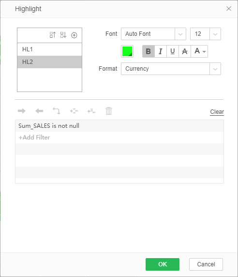
3. set HL2: bold font, font color, background color were green and white, the format is set to currency, set the filter condition to "Sum _SALES" is not "null", as shown below.

4. The result after highlighting the application is shown in the figure below. "Sum_SALES" is an empty cell, filled with the number 0 in the font color red, the background of the cell that is not empty is displayed in green, the font is bold in white, the Chinese currency is added before the number (and the current environment Language is consistent).